g2sys

Discovering static and dynamic coupling in a set of sensors.

---

g2sys leverages the plars module presented in the previous sections in order to exhibit multi-variate polynomial¹ relationships involving a set of sensors’ time-series included in the training dataset.

Let us first state the problem the g2sys is designed to address before we go deeper in the presentation.

1 Problem statement

g2sys is a graphical user-friendly interface (GUI) which enables an easy and efficient manipualtion of the parameters defining the structure of relationhips² in order to discover invariant relationships between a set of sensors and their delayed values.

Moreover, the GUI enables to choose the training regions and show the residuals associated to the discovered relationships over the whole dataset. This enables to check their generalization powers (the persistence of their invariance).

Let us first of all precisely define the class of relationships g2sys helps discovering.

Regardless of the kind of a relationhip (see below), the latter is always associated to a sensor index, say \(i\).

The relationship is then expressed in one of the following two forms:

Static

\[ s_i(k)=F_i\left(\{s_j(k-\sigma\times d_i)\}_{(j\neq i,\sigma\in \{0,\dots,m_i\})}\right) \tag{1}\] \(\rightarrow\) \(s_i\) is a static function of the other sensors and their past values up to \(m_i\times d_i\).

Dynamic

\[ \bigl[\Delta^{(m_i)} s_i\bigr](k)=F_i\left(\begin{array} \{s_i(k-\sigma\times d_i)\}_{\sigma\in \{1,\dots,m_i\}}\cr \{s_j(k-\sigma\times d_i)\}_{(j\neq i,\sigma\in \{0,\dots,m_i\})} \end{array} \right) \tag{2}\] \(\rightarrow\) The increment \(\bigl[\Delta^{(m_i)} s_i\bigr](k)\) represents the discrete version, at instant \(k\), of the \(m_i\) derivatives of \(s_i\).

In the following sections, the two classes of relationships are detailed.

2 The classes of relationships

Depending on the parameters setting of the g2sys module, the following two kinds of polynomial relationships might be targeted by the search engine:

2.1 Static relationships

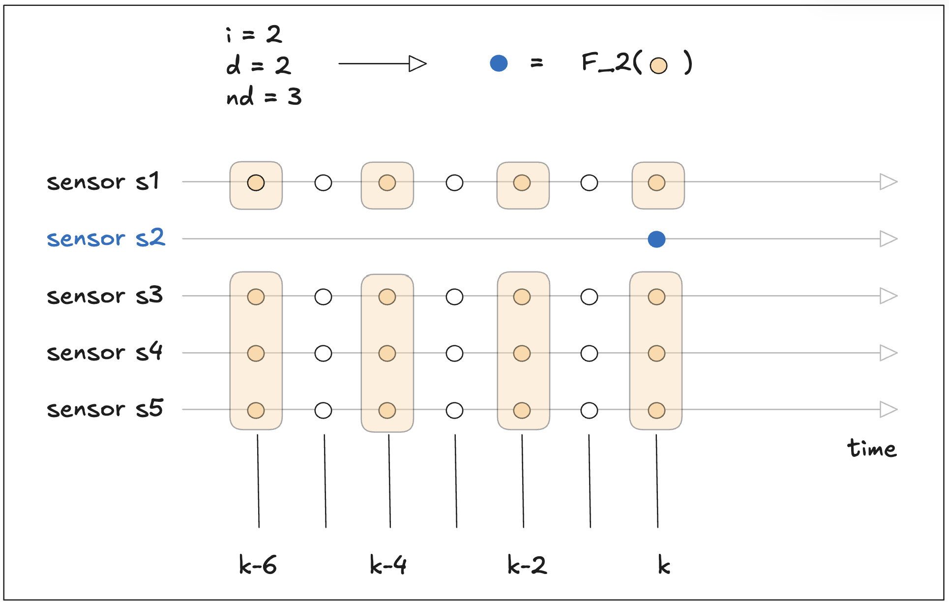
In a static relationship, related to sensor index \(i\), the st of arguments of the polynomial \(P_i\) involved in Equation 1 is given by:

\[ \texttt{(Static)}\quad \texttt{arguments of $P_i$}: \quad \begin{bmatrix} s_j(k)\\ s_j(k-d)\\ \vdots\\ s_j(k-n_d\times d) \end{bmatrix}_{j\neq i} \tag{3}\] Namely, all the values of all the sensors, except \(i\), and their delayed version, with \(n_d\) multiples of the delay \(d\). This relation is named static because the previous values of the label (sensor \(i\)) are not involved in the vector of features.

Regarding the design parameters \(d\) and \(n_d\)

The elementary delay \(d\in \mathbb N\) as well as the number of delays considered in the arguments of \(P_i\) are two of the search parameters (see below).

Notice that when choosing \(d>1\), an under-sampling is applied which can be necessary in many cases where a high sampling rate is present in the data that is not necessarily useful³ for the relationships’ discovery.

Based on the above definitions, the static relationships can be schematically described by the following figure:

Figure 1: Illustration of the logic of a static relationship indexed by sensor 2 with \(n_d=3\), \(d=2\).

2.2 Dynamic relationships

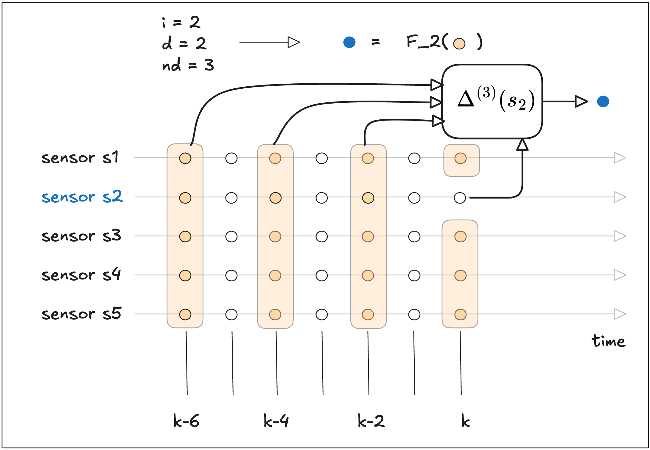
The dynamic relatioships might possibly⁴ correspond to discrete versions of any possible differential relationships expressed via multi-variate polynomials.

Mathematically, such relationships involve arguments of the form expressed by Equation 3 with a major difference in that the index \(j\) spans all sensors indices including the index \(i\) of the targeted sensor with only one exception, namley the value \(s_i(k)\).

Moreover, keep in mind that, in the case where only one delay is used \(n_d=1\), the relationship should approximate the increment \[\Delta^{(1)} s_i(k):=s_i(k)-s_i(k-d)\] rather than the simple value \(s_i(k)\). In the case where two increments are used \(n_d=2\), the target becomes:

\[ \Delta^{(2)} s_i(k):= s_i(k)-2s_i(k-1)+s_i(k-2) \]

and so on for the higher values of \(n_d\in \mathbb N\).

This can be schematically represented in the following figure:

Figure 2: Illustration of the a dynamic relationship associated to \(i=2\), \(d=2\) and \(n_d=3\).

3 Redundancy & implicit character

In this section, some important aspects that are worth keeping in mind when using g2sys are briefly discussed.

3.1 An illustrative example

As a supporting example, let us consider the following relationship linking tow sensors:

• The speed \(v\) of a vehcule of mass \(m\) and
• The acceleration pedal’s angular position \(\theta\).

Let us assume that an angular position \(\theta\) induces a traction force \(T=K\theta\) that is proportional to \(\theta\) and that a friction term given by \(-\lambda_f v^2\) is present. The Newton’s law can be written as follows:

\[ \dfrac{dv}{dt} = K\theta-\lambda_f v^2 \tag{4}\]

In this example, let us assume that we dispose of two sensors:

\[ s_1=v\quad \text{and}\quad s_2=\theta \]

Let us try to analyze what happens when we try to exhibit (discover) relationships when successively using \(i=1\) and \(i=2\).

3.1.1 Case where \(i=1\)

In this case, one is targetting relationships on the sensor \[s_1=v\] As mentioned, above this can be static or dynamic.

3.1.1.1 Static relationships

In this case, using \(n_d=1\), one is looking for a relationship of the form:

\[v_k=P_1(\theta_k, \theta_{k-d}, \dots, \theta_{k-n_d\times d})\]

which is obviously non existant. One cannot guess the speed of the vehicle from the recent history of the angular position of the acceleration’s pedal.

3.1.1.2 Dynamic relationships

In this case, one is looking for a relationship of the form:

\[v_k-v_{k-d}=P_1(v_{k-d}, \dots, v_{k-n_d\times d}, \theta_k, \theta_{k-d}, \dots, \theta_{k-n_d\times d})\]

But we know from Equation 4 that we have (approximately):

\[ \dfrac{v_{k}-v_{k-d}}{d\times \tau} = K\theta_k -\lambda_f (v_{k-d}^2 + \varepsilon_k)\quad \text{where}\quad \varepsilon_k:=(v_k^2-v_{k-d}^2) \] where \(\tau\) stands for the sampling acquisition period.

This means that a dynamic relationship can be approximately found provided that the speed of the vehicle⁵ is slowly varying or the sampling time is sufficiently small.

To summarize, in this case, a dynamic relationship would be found for which the polynomial present in the r.h.s of Equation 1 is given by:

\[ P_1(\cdot) = (d\times \tau)\times (K\theta_k-\lambda_f v_{k-d}^2) \tag{5}\]

3.1.2 Case where \(i=2\)

Now what happens when using \(i=2\) which considers the target sensor to be \[s_2=\theta\qquad ?\]

3.1.2.1 Static relationships

Stranglely enough, this is much simpler since the static form of Equation 1 can be identified leading to:

\[ \theta_k \approx P_2(\cdot):=\dfrac{1}{K}\times \Bigl[\dfrac{1}{d\times \tau}(v_k-v_{k-d})+\lambda_f\times v_k^2\Bigr] \tag{6}\]

which simply expresses the fact that the acceleration pedal’s angular position can be expressed in terms of the speed and its delayed value.

3.1.2.2 Dynamic relationships

Obviouly Equation 6 when written at instants \(k\) and \(k-1\) enables to write:

\[ \begin{align} \theta_k-\theta_{k-d} = &\dfrac{1}{K}\times \Bigl[\dfrac{1}{d\times \tau}(v_k-v_{k-d})+\lambda_f\times v_k^2\Bigr] \\ &+ \dfrac{1}{K}\times \Bigl[\dfrac{1}{d\times \tau}(v_{k-d}-v_{k-2d})+\lambda_f\times v_{k-d}^2\Bigr] \label{encoreundyntheta} \end{align} \tag{7}\]

which is another representation of the same physical law Equation 4 that can be obtained provided that \(n_d\ge 2\) is used.

Therefore, the statement of the next section should be kept in mind.

3.2 Keep in mind

The previous simple example illustrates the following statement that should be kept in mind when usingg2sys tools:

keep in mind

Fact1

The same physical law might lead (or lie behind) several relationships that can be discovered by g2sys. Some of the latter can be static while others are dynamics.

Fact2

The wording static or dynamic is totally linked to the targeted sensor \(i\): A static relationship for sensor \(i\) contains only \(s_i(k)\) in the left hand side of the relationship while \(\Delta^{(n_d)}(s_i)(k)\) appears in the l.h.s of dynamic relationships.

BUT static relationships might involve dynamic⁶ terms in the r.h.s as it is the case in Equation 6 and Equation 7.

4 The importance of scalability

The number of original variables (before polynomial expansion) that results from the choice of the number of delays \(n_d\) is equal to:

\[ n = (n_d+1) \times (\text{number of sensors}) \]

Recalling that it is a polynomial expansion of these variables that is to be searched for, it appears clearly that the scalability of the sparse solver becomes rapidly quite important in order to handle realistic industriel problems. (See the discussion on the cardinality of multi-variate polynomials which is analyzed in the introductiont to the plars module.)

Footnotes

1. Refer to the polynomial’s dedicated section for the precise definition.

2. This includes the degree of the polynomials, the delays introduced (their amounts and numbre) as well as the precision of the solutions, the thresholds on the monomial conributions to cite only a part of the degrees of freedom.

3. It can even be harmful in the presence of relatively high noise in the measurements.

4. Provided that the parameters \(n_d\) and \(d\) are correctly tuned.

5. As present in the training dataset.

6. Expression derivatives of other sensors.