g2sys
Principle
1 The two form of g2sys module
The g2sys module comes with in two different forms, both using the same core computation module:
A Graphical User Interfance (GUI) which is
streamlit-powered application that facilitates the choice of the parameters.A standard python module that can be used inside a python script.
A standard workflow might be to use the streamlit version to find the approriate set of paramaters for each targeted label and once the setting is found, use it in the script version to produce the personalized results and outputs.
More details regarding these two forms are given in the API documentation section
2 Computation architecture
The principle of the g2sys module is depicted in Figure 1 below
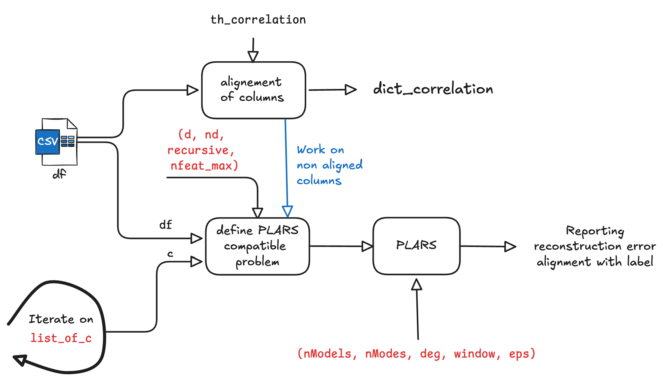
plars algorithm as described by the arguments shown in red.
Notice the following facts:
The set of alignments between columns is reported in a dictionary of correlations. Only uncorrelated columns are used in the search for relationships. This reduces the computational burden by avoiding establishing easy-to-detect relationships on the one hand and reduce the number of eligible monomials in the relationshops one is looking to establish.
Obviously, later on, the normality assessment process must also investigate whether previously aligned columns are still ligned, otherwise a missing alignement flag should be raised as this might be induced by a default in the equipment.
For each of the remaining non aligned sensors, a
plars-compatible problem (see the introductory section for g2sys) and the associated regression problem is solved and the results are reported for the user’s convenience.Notice that the creation of the plars-compatible regression problem needs the parameters
d,ndandrecursiveto be defined.- The
recursiveboolean optionThe recursive parameters is used to inform whether it is a static or a dynamic relationship that is searched for. More precisely, setting
recursivetotruemeans that a dynamic relationship is searched for, otherwise, a static relationship is targeted (see the related definitions for a recall regarding the definition of these modes). The operation is repeated over the list of sensors to be investigated. This list is designated by the input argument
list_of_c.
3 Sparsity enhances reliability & interpretability
While the crucial role of sparsity in addressing false alarm and anomaly detection has been previously underlined in the Parsimony-related chapter and the examples that follow. It is worth mentioning it again in this g2sys -related chapter by addressing more realistic examples while underlying a new advantage that is associated to the interpretability issue.
3.1 Reliability
It is important to understand the role of sparsity in providing reliable and interpretable anomaly detection because sparsity lies in the very heart of the MizoPol package.
3.1.1 A real-life example
In order to understand this key issue, we shall invoke the results shown in the use-case presented in the metro compressor section where a system representing a train’s compressor (15 sensors) is analyzed by means of the g2sys dedicated Graphical User Interface (GUI).
After few clicks and iterations, it is shown that a tight static relationship can be found indexed by the sensor called Reservoir. The model has been fitted using only 12% of the learning data.
The following figure shows a screenshot of the GUI after these manipulations.
The bold title of the figure states the following facts:
The model involves only \(5\) monomials (hence, \(5\) coefficients).
It provides a very small regression error and an almost perfect alignment
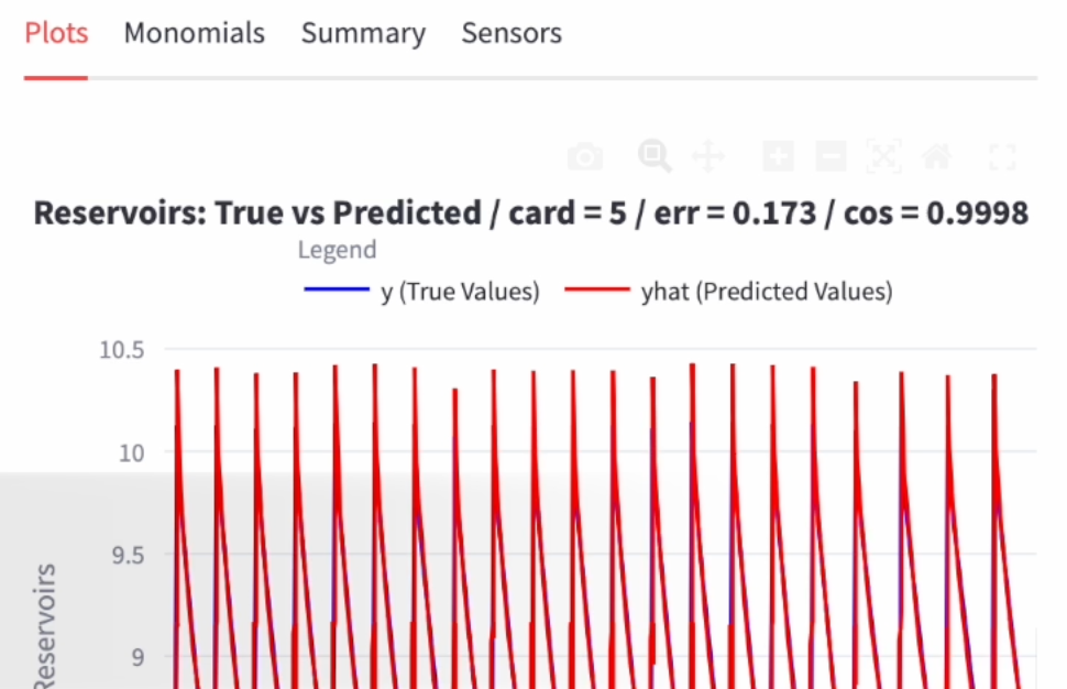
g2sys GUI showing some information regarding the identified polynomial and the regression quality of the sensor/label \(\texttt{Reservoirs}\).The next figure shows the examination through the GUI of the residual (the normalized regression error) between the truly measured value of the \(\texttt{Reservoirs}\) sensor and the one provided by the fitted sparse polynomial:
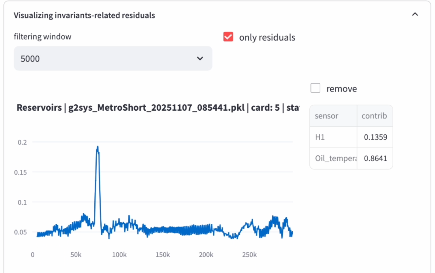
This figure suggests the following observations:
- The relationship links the sensor defining the label, namely \(\texttt{Reservoirs}\) to the two sensors: \(\texttt{H1}\) and \(\texttt{Oil\_temperature}\) so that one can write:
\[ \texttt{Reservoir} = P\Bigl(\texttt{H1}, \texttt{Oil\_temperature}\Bigr) \tag{1}\]
where \(P\) is a polynomial with only \(5\) monomials as discussed above.
Based on the previous fact, let us consider the following question:
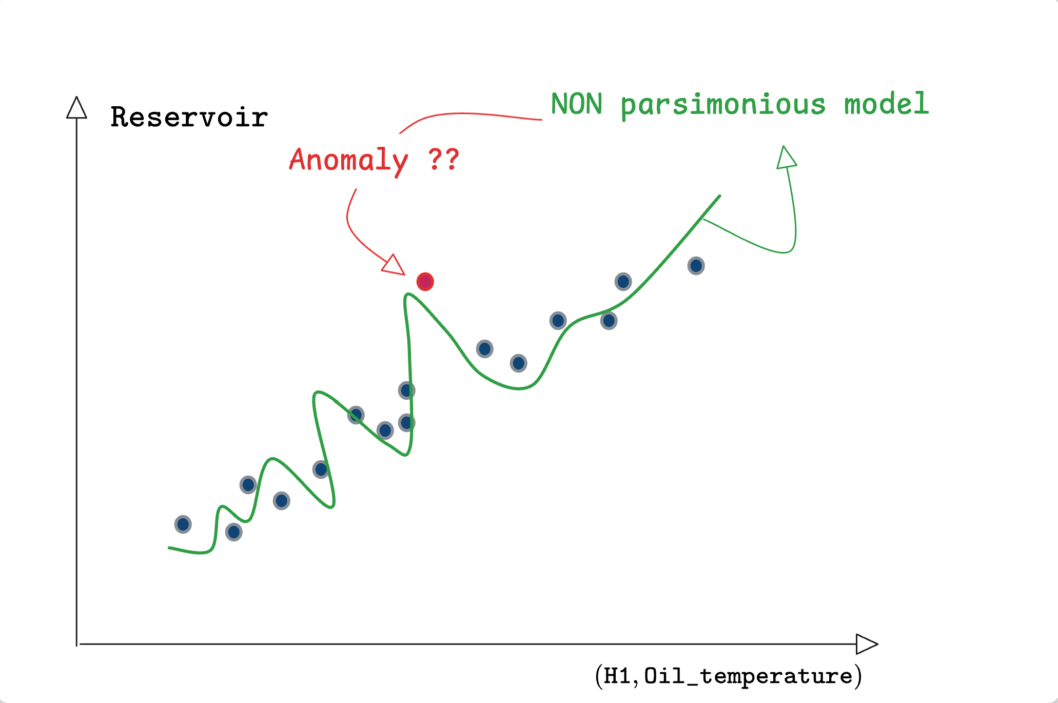
What are the odds that a model with only 5 parameters fits with an error lower than 7% over almost all the 300,000 instances while reaching 20% consistently over a small interval (see Figure 2) without this interval representing one of following two possibilities affecting the triplet \[(\texttt{Reservoir}, \texttt{H1}, \texttt{Oil\_temperature})\]
Either a context that is not seen in the training data
Or a true anomaly affecting the compressor that disturbed the relationship between these three sensors?
The odds should be very small but the answer would not be so straightforward should the model be a Deep Neural Network with 200,000 parameters that densly links all the existing sensors.
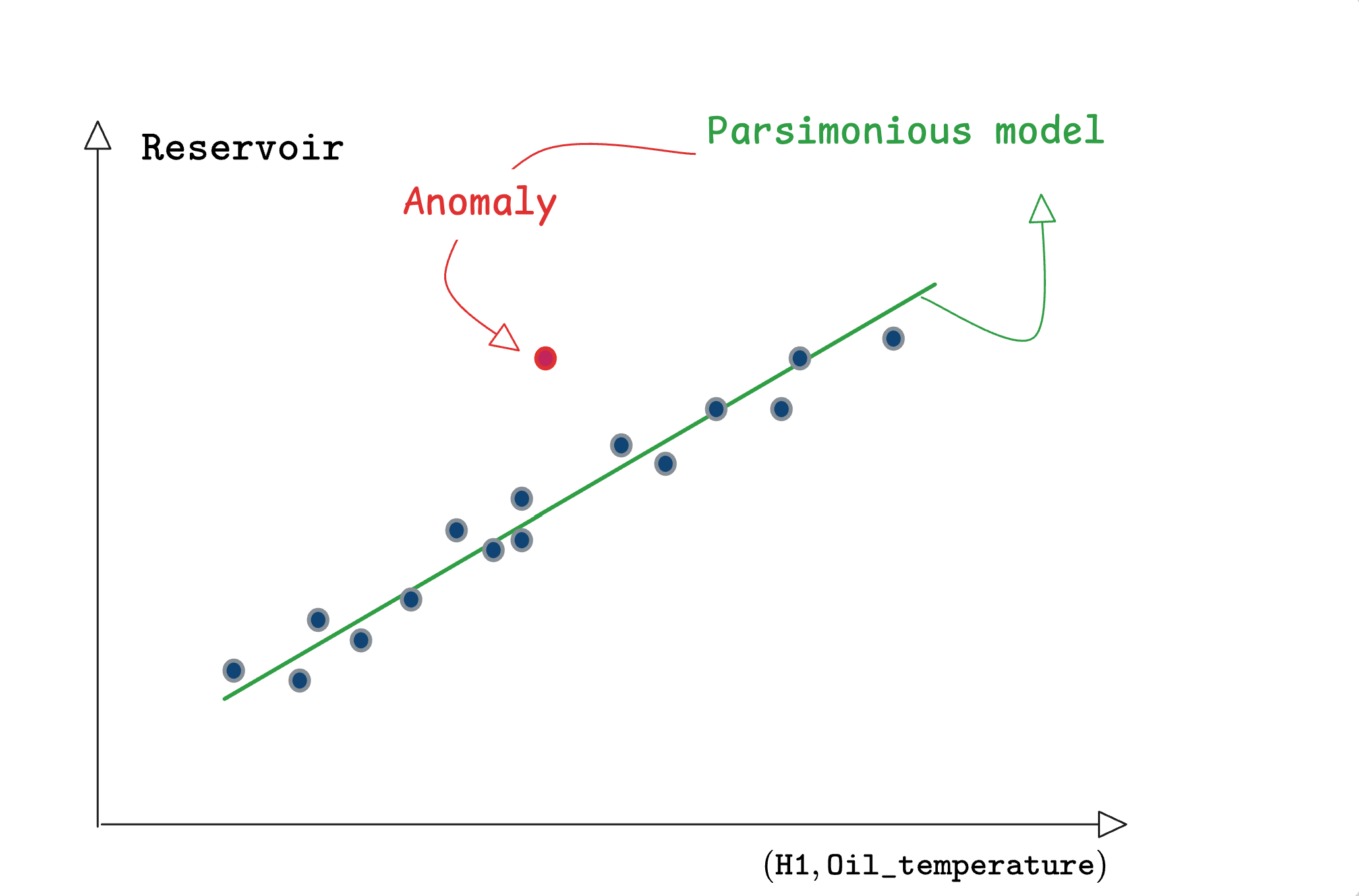
3.1.2 A sketchy example
If this is not yet clear, the following two tabs hopefully might help:
3.2 Interpretability
The discussion of the previous section was centered on reliability: sparsity makes decision reliable as the characterization of normality is less prone to overfitting and mis-representation.
But what about interpretability?
Let us consider again the example of the train compressor system used in Section 3.1.1 above. Recall that our dataset involves 15 sensors meaning that if we use an anomaly detection method that provides a black-box like anomaly-related residual, it would be difficult to interpret this residual having high value1. One can just states that there is something wrong happening.
On the contrary, the fact that the residual is defined by the error on Equation 1 leads naturally to the following diagnosis:
There is an anomaly that is linked to the triplet:
(\(\texttt{Reservoir}, \texttt{H1}, \texttt{Oil\_tempoerature}\)),
namely:
Either at least one of these sensors is deficient (but this should therefore be seen in all sparse relationships that involves this sensor)
Or their relationship is detuned for whatever reasons that the operator would recognize quite rapidly once she is notified that the default lies in this set of three sensors.
Another very speaking example showing the role of the sparsity in enhancing both the reliability of the diagnosis and its interpetability is given through the use-case of the section dedicated to the hydraulic system.
For the time being let us emphasize the need for delays when looking for relationships in some use-cases.
Footnotes
There are some alternatives but franckly, they are not reliable nor trustworthy.↩︎