Overview
The mizopol suite in a glance.
The mizopol suite currently consists of the following modules that are presented in details through this documentation.
The presentation below aims at giving a brief and sketchy overview of the tools.
The script provided in the sketchy presentation uses the local version of the packages. For a precise and rigorous syntax of the publicly available API, refer to the API-documentation section below.
1 plars
Identify a sparse multi-variate polynomial1 \(P\) such that: \[y\approx P(x)\]
The algorithm is based on a modified, scalable version of the LARS (least angle) algorithm.
The plars module is detailed here.
M. Alamir, Nonlinear control of uncertain systems: conventional and data driven alternatives with python. Springer-Nature, November, 2025
Notice that plars is the fundamental building brick of the whole package in the sense that all the other modules call it at some stage of their execution.
2 g2sys
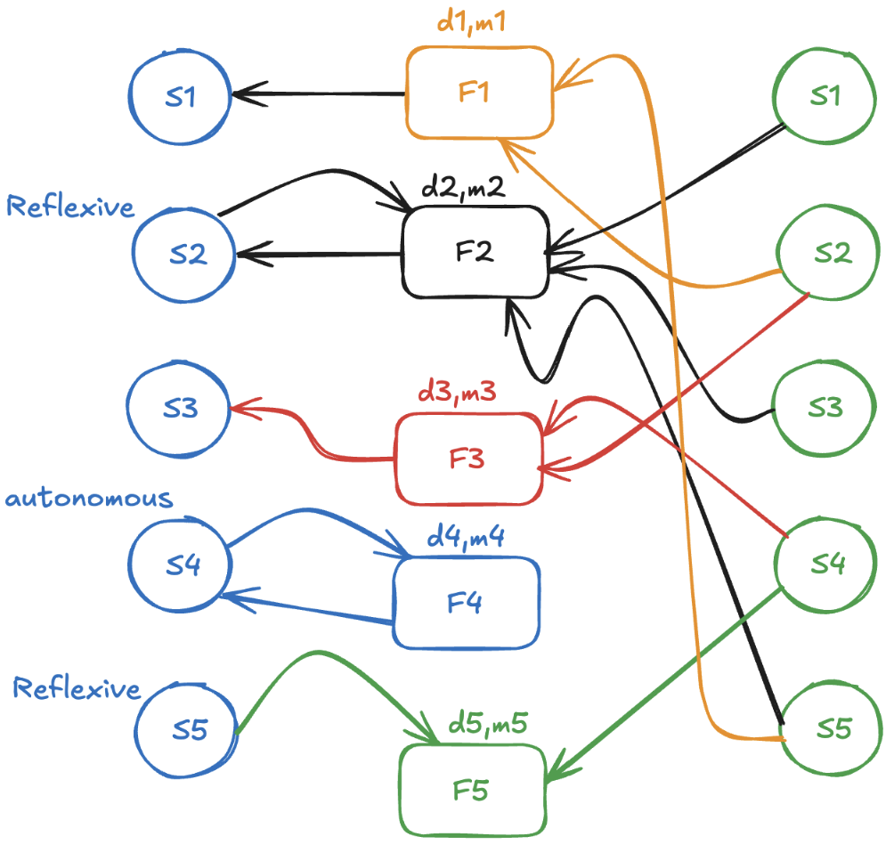
Given sensors \(s_1\), …, \(s_n\), fit a set of relationships of one of the following two forms:
\[ s_i(k)=F_i\left(\{s_j(k-\sigma\times d_i)\}_{(j\neq i,\sigma\in \{0,\dots,m_i\})}\right) \] \(\rightarrow\) \(s_i\) is a static function of the other sensors and their past values up to \(m_i\times d_i\).
\[ \bigl[\Delta^{(m_i)} s_i\bigr](k)=F_i\left(\begin{array} \{s_i(k-\sigma\times d_i)\}_{\sigma\in \{1,\dots,m_i\}}\cr \{s_j(k-\sigma\times d_i)\}_{(j\neq i,\sigma\in \{0,\dots,m_i\})} \end{array} \right) \] \(\rightarrow\) The increment \(\bigl[\Delta^{(m_i)} s_i\bigr](k)\) represents the discrete version, at instant \(k\), of the \(m_i\) derivatives of \(s_i\).
Can be use to achieve the following tasks:
- Design explainable normality indicators
- Discover unmodelled relationships
- Help designing Dynamic Digital Twins
- Detecting contexts in the datasets
- Remove redundant sensors
- Survey persistant correlations
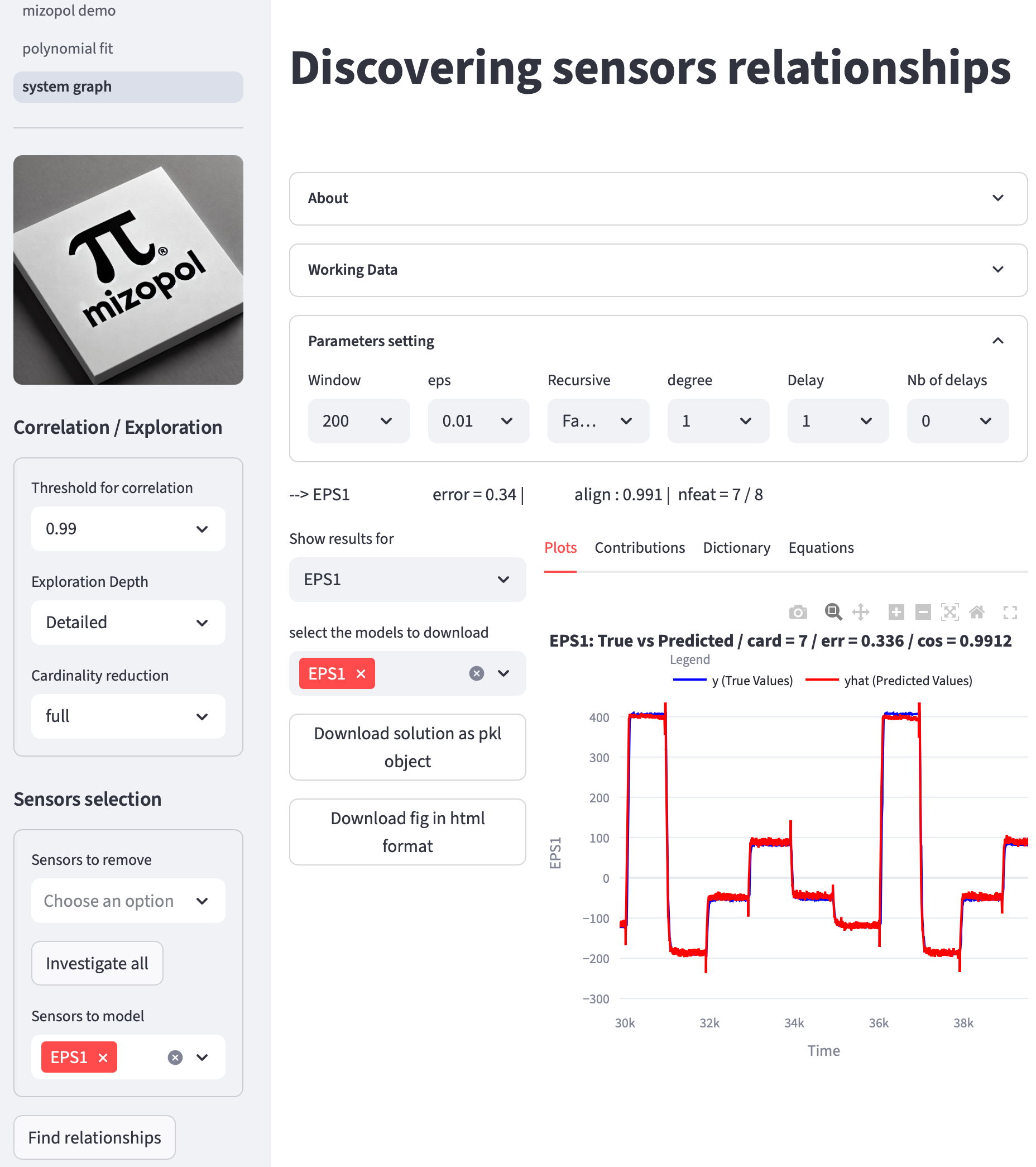
The g2sys module is detailed here
static, dynamic etc.3 pwpol
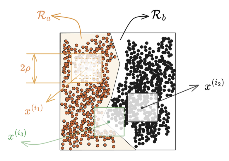
Given a set of sensors \(s_j\), \(j=1,\dots,n_s\) and a target sensor \(s_i\), find a set of \(n_r\) polynomials \(P_\sigma\), \(\sigma=1,\dots,n_r\), such that the following residual: \[ e_i = \min_{\sigma=1}^{n_r}\Bigl\vert s_i-P_\sigma(\{s_j\}_{j\neq i})\Bigr\vert \tag{1}\] is small.
Notice that:
Equation 1 defines an implicit invariant describing the normality of the system should the dataset on which it is computed be healthy.
The number \(n_r\) of polynomials should be made as small as possible.
Equation 1 does not provide a prediction capability since the residual can be computed only when the measurement \(s_i\) is available.
The pwpol module is detailed here.
pwpol module.4 xpwpol
This module builds on the previous one, namely pwpol in order to provides an explicit piece-wise polynomial representation. More precisely, this is done in two steps:
First an impicit piece-wise polynomial representation is obtained by using
pwpol. This provides the set of polynomials \(P_\sigma\) mentioned in Equation 1.Then the new tools available in
xwpolworks on the above resulting set in order to provide an explicit representation of the form:
\[ \hat y = \dfrac{1}{n_v} \sum_{\kappa=1}^{n_v}P_{\sigma(x\vert \kappa)}(x)\quad \text{where}\quad \sigma(x\vert \kappa)\in \{1,\dots,n_r\} \tag{2}\]
where \(n_v\) is an integer representing a number of voters while \(\sigma(x\vert i_v)\) is the index of the selected polynomial at the vector of features \(x\) for the \(i_v\)-th voter.
More detailed are provided in the xpwpol-dedicated section.
5 rlars
Given
- a features vector \(x\) and
- a label \(y\),
find a set of multi-variate polynomials:
\[ c_0(x),\dots, c_r(x) \]
such that \(y\) is a root of the following scalar polyomial (in the unknown \(z\)):
\[ c_r(x)z^r+\dots+c_1(x)z+c_0(x) \]
More precisely, the following can be viewed as a residual for the normality characterization of the pair \((x,y)\):
\[ R(x,y):=\sum_{j=0}^rc_j(x)y^j \tag{3}\]
The starting point of this structure is that in the particular case where \(r=1\), Equation 3 simply implies that: \[ y = -\dfrac{c_0(x)}{c_1(x)} \]
which is simply a multi-variate fractional expression in the features vector \(x\).
This generalizes the polynomial structure targeted by plars.
Notice however that this is only the starting point, the results obviously offer a much wider generalization than simply fractional representation when \(r>1\).
6 Undergoing research
MizoPol is a research-steered package. New features and modules are expected to be added continuously as the research goes.
Footnotes
see the polynomial page for a rigorous definition.↩︎