Piece-wise polynomials
On the rationale behind and the explicit/implicit forms of piece-wise polynomial residuals and their potential use.
In this section, we discuss the class of piece-wise polynomial relationships, in their implicit and explicit forms.
But let us first justify the reason for which these relationships might be of great help in characterizing the normality in industrial time-series and hence in detecting unmodelled anomalies in industrial equipments.
1 Why?
Although multi-variate polynomials relationhips cover a wide class of physical laws, it is obvious that they do not cover every possibility. Think about the relationship involving trigonometric functions, square roots, exponential or rational relationships1.
However, any smooth relationship can be represented by region-dependent polynomials, namely:
the feature space is partitioned into a set of regions over each of which a polynomial relationship captures the dependencies that hold on that specific region.
In the industrial context, the regions mentioned above can be the result of different contexts of use that might encompass different tunings of controller, different values of the set-points (which might be absent from the set of measurement contained in the dataset) or different configurations of the system.
2 Examples
One can simply think about a controlled system that tracks some reference signal \(\texttt{y\_ref}\) and depending on the error \(e=y-\texttt{y\_ref}\) between the regulated signal \(y\) and that reference \(\texttt{y\_ref}\). In order to avoid overshoots, it is common to define a gain scheduled feedback which applies a control voltage, say \(u\) which is propotional to the error with a proportional gain \(K\) that is:
- High when small tracking errors are measured and
- Low when high tracking errors are measured.
Namely
\[ u = \left\{ \begin{array}{ll} -K_h\times e\quad & \text{if $\vert e\vert \le \epsilon$}\\ -K_\ell\times e\quad & \text{otherwise}\\ \end{array} \right. \tag{1}\]
This obviously splits the space (via the condition \(\vert y-\texttt{y\_{ref}}\vert\le \epsilon\)) into two regions over each of which the relationship between the features \((y,\texttt{y\_ref})\) and the targeted label \(u\) is polynomial (linear in the specific example) but there is no a single polynomial relationship that matches Equation 1 on the whole space of features.
This example is quite simple compared to industrial context where so many parameters might be involved in the definition of the so-called context. The latter is rarely available to the engineer in charge of designing anomaly detection algorithms. This means that:
The normality characterization algorithm should be unaware of the parameters that defines the context (the different regions of smooth relationships). The piece-wise relationships should be built without the knowlege of the precise definition of the unknown region.
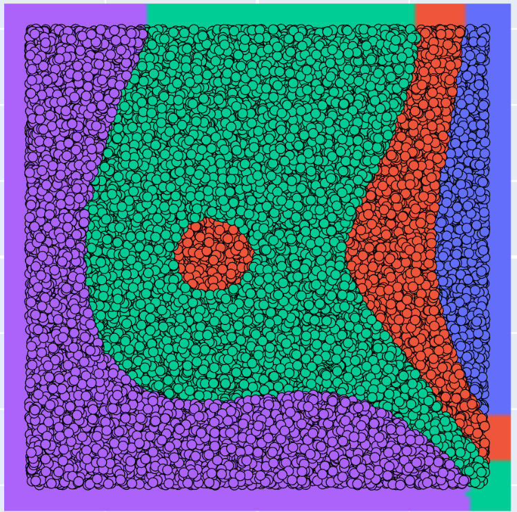
The figure aside shows another examples that comes from the Kaggle dataset dedicated to the parameteric anomaly detection in time-series.
Over each of the four regions, a sensor \(y\) depends on the features vector \(x\in \mathbb R^2\) through different polynomials, namely:
\[ y = P_i(x)\quad x\in \mathcal R_i\quad i\in \{1,\dots,4\} \tag{2}\]
Beside the examples discussed above which are induced by the presence of different operational modes, the need for piece-wise polynomial structures can be triggered by the need to approximate non rigorously polynomial relationships between the sensors involved.
3 Explicit form
When the region is known, namely when it is possible, knowing \(x\) to associate the index \(i\) of the region as shown in Equation 2, the relationship is called explicit piewe-wise polynomial.
More precisely, in the case of explicit piece-wise relationships, there exists a known integer values map \(i^\star\) such that for a given \(x\), \(i^\star(x)\) denotes the index of the region to which belong the features vector \(x\):
\[ x\in \mathcal R_{i^\star(x)} \tag{3}\]
In this case, the relationship Equation 2 enables to predict the value of the label \(y\) for a given value of the features vector \(x\). The normality is then associated to the so-called prediction error given by:
\[ e = \mu\Bigl(\overbrace{P_{i^\star(x)}(x)}^{\hat y(x)}-y\Bigr) \tag{4}\]
Although the explicit piece-wise polynomial form is even larger than the explicit single unique polynomial form, it is sometimes hard to find for the reasons invoked in the following section.
3.1 The need for an implicit form
Unfortunately, as it has been mentioned earlier, it is not always possible to identify the region’s index map Equation 3 in real-life situations. There are two reasons for this impossibility:
The first lies in the difficulties associated to the identification of the classifier represented by the index region map \(i^\star(x)\) even when it factually exists.
More importantly, it is possible that there is no explicit relationship between the feature vector \(x\) and the label \(y\) because the information contained in \(x\) is not complete.
This is the case for instance when the true hidden relationship that governs \(y\) takes the following form:
\[ y = F(x, z)\quad \text{$z$ not available} \]
where \(z\) is a context variable having a finite set of unknown values that do not uniquely depend on the vector \(x\) of features2. Obviously, since in this case, the context does not depend on the features, it is impossible to identify the index map from the sole knowledge of \(x\) as \(z\) which is a crucial information that is needed to define the region, is simply not available.
Here is where the implicit form of the piece-wise relationships enter into the scene. This is explained in the next section.
4 Implicit form
In the implicit form of the normality characterization via piece-wise polynomial relationships, the residual is defined by the following equality:
\[ e = \min_{i=1}^{n_r} \left\vert y - P_i(x)\right\vert \tag{5}\]
where \(n_r\) is the number of multi-variate polynomials that are involved in the implicit relationship.
It is important to notice that:
The relationship Equation 5 that determines the residual \(e\) expresses the distance of the measurement \(y\) to the closest value among the set of values provided by the set of polynomials at \(x\), namely:
\[\text{Set of values of the implicit model at $x$}\qquad \Bigl\{\hat y_i(x):=P_i(x)\Bigr\}_{i\le n_r}\]
There is no way to compute the predicted value of \(y\) (by the model) before the true value of \(y\) is known.
In other words, in the absence of \(y\), there is no way to determine which one of the values \(P_i(x)\) is the closest to the true value \(y\). Nevetheless, whey \((x,y)\) is available, a residual (distance to normality) can be computed by Equation 5.
This is why the implicit relationships are mainly used to characterize the normality and hence to raise alarms when the residual goes beyond some pre-defined threshold.
The explicit form might be used for both anomalies detection and digital twin enhancement. But the latter is less common to be found.
5 All the identification are parsimonious
In the above discussion, we did not recall the fact that:
whether they are implicit or explicit, the polynomial relationships that are identified by the modules of the MizoPol suite are all parsimonious.
The reasons for which parsimony is a key element in the context of processing industrial and technological time-series are discussed in the parsimony-dedicated section.
Footnotes
Notice however that if these non polynomial maps are a priori known, a virtual components might be added to the vector of features \(x\) so that the standard polynomial structure become appropriate to capture the originally non polynomial relationships. But we do not consider this case here.↩︎
Think about a robot performing a set of different tasks involving pieces of different weights and/or moments of ineria.↩︎