rlars
Illustrative example on the twin-pendulum system
1 The system
In this section an example of use of the rlars module is provided where it is used to characterize the normality via a reduced number of short experiments.
The system consists in two pendulums that share the same axis of rotation that is fixd on a moving cart. The only possible exogenous action is provided by the horizontal driving force applied to the cart.
It is assumed that the model is not known so that very sophisticated (and rationla) actions that would enable a rich exploration of the state space are not available. Only short and rapidly damped experiments are tolerated.
See this funny video regarding the control of this system (should its model be known which is not the case in the present study).

rlars is used in order to characterize the normality from a reduced number of samples.2 Experiment design
An excitation generator function is designed that produces signals composed of nModes frequencies uniformly distributed on the interval \([0,\texttt{omega\_max}]\) and damped with an exponential decay rate of mu.
This is expressed in the following python function which returns a function of time representing the candidate excitation that is defined in a random way:
def create_udet(u_max, omega_max, nModes, mu):
    '''
    Facility that creates a function of of the time
    that provides the control to be applied at the instant
    used as argument.

    u_max       : the maximum value of the control ampllitude
    omega_max   : the maximum pulsation used in the excitation signal
    nModes      : the number of modes from 0 to omega_max
    mu          : The decrease rate of the signal.
    '''
    omegas = np.linspace(0, omega_max, nModes)
    coeff = np.random.randn(nModes)
    angle = np.random.rand(nModes) * 2 * np.pi
    M = lambda t: np.array([np.sin(omegas[i] * t +angle[i])
                            for i in range(nModes)])
    def udet(t):
        v = np.sum(M(t) * coeff) * np.exp(-mu * t) * (u_max/3)
        return min(u_max, max(-u_max, v))

    return udet
The following figure shows three different resulting excitation profiles that mainly last around one minute each (you can zoom on the figure to closely examine the evolution in time):
3 Working dataset
The following steps have been used to built the working datasets:
Four different experiments are simulated using four different random excitation profiles as defined in the previous section.
In order to emulate the presence of mechanical stops limiting the linear movement of the cart, each simulation has been truncated from the instant where the stop is reached (the stops are positioned at \(r_{max}=\pm 100\)).
Given that the sampling period for the measurement acquisition is set to \(\tau=0.01\) sec, the total available samples should the previous truncating step be avoided would have been equal to 20,000. As a matter of fact the truncation leads to a total dataset containing 11,822 samples.
Although the model is supposed to be unknown, it can be reasonably assumed that the underlying laws are defined in terms of the second derivatives:
\[ y_1 = \ddot{\theta}_1 \quad,\quad y_2 = \ddot{\theta}_2 \quad,\quad y_3 = \ddot{r} \]
being functions of the features vector:
\[ x = \begin{bmatrix} r & \dot r & \theta_1 & \dot{\theta}_1 & \theta_2 & \dot\theta_2 & u & \sin\theta_1 & \cos\theta_1 & \sin\theta_2 & \cos\theta_2 \end{bmatrix} \in \mathbb{R}^{11} \]
That is the reason why building the features matrix and the label vectors is completed using the python module
ml_derivatives, which provides a robust reconstruction of the derivatives of noisy time series see Alamir (2025) and the module description.5% noise added before computing the high derivativesIn order to emulate real-life noisy conditions, a relative white noise has been added with a standard deviation of 5% of the 95th percentile of each of the simulated profiles \(\theta_1\), \(\theta_2\), and \(r\).
These noisy versions are used in the reconstruction of the derivatives and hence in the resulting working dataset.
4 Identification results | comparison to plars
In order to highlight the advantage of using the rlars module over the simple use of plars, we first show the identification results when using the latter.
As far as the normalized error is concerned, it is defined as a ratio of the \(95%\)-quantile of the residual to the median of the norm of the label, namely:
\[ \texttt{normalized error}= \dfrac{\texttt{percentile}(\texttt{residual}, 95)}{\texttt{median}(\vert y\vert)} \]
4.1 plars (explicit polynomials)
The following script and dataframe showing the statistics of the normalized error when multi-variate polynomial’s identification is attempted via the plars module.
from mizopol.plars_api import predict, fit
import pandas as pd
from sklearn.model_selection import train_test_split


dic_args = dict(
    window=1000
    deg=3
    nModels = 40
    nModes = 20
    eps = 0.02
    test_size=0.1
)

dic_plars_fit = dict(
        compute_contributions=False,
        colNames=[f'S{i + 1}' for i in range(X.shape[1])],
        nfeats=None,
    )

panel_plars = []

i = 1
for z in [y1, y2, y3]:

    Xid = (X-X.mean(axis=0))/X.std(axis=0)
    Xtrain, Xtest, ytrain, ytest = train_test_split(Xid, z,
                                    test_size=test_size,
                                    shuffle=False)

    solution, _ = fit(Xtrain, ytrain, dic_args, dic_argsFit)

    print(f"plars solution's cardinality for y{i} = {solution['card']}")
    dfi = solution['dfe_train']
    dfi.columns = [f'Error on y{i}']
    i += 1
    panel_plars.append(dfi)

dfRes_plars = pd.concat(panel_plars, axis=1)
dfRes_plars
plars solution's cardinality for y1 = 251
plars solution's cardinality for y2 = 256
plars solution's cardinality for y3 = 237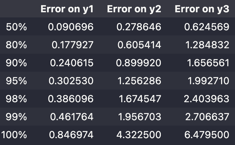
These results are those obtained on the train data. They are sufficiently bad to make the examination of the result on test data useless.
4.2 rlars: (labels as polynomials’ roots)
In this attemps, we use the same parameters except the degree that is reduced to deg=2 in order to emphasize the fact that the underlying strucutre is sufficiently rich for a lower order model to capture the relationships drastically better that the polynomial even with lower degree.
from mizopol.rlars_api import fit, predict
import pandas as pd
from sklearn.model_selection import train_test_split

dic = dict(deg=2, window=1000, nModes=40, nModels=20, eps=2e-2)

dic_fit = dict(
    colNames=[f's{i + 1}' for i in range(nx)],
    compute_contributions=True,
    nfeats=None,
    th_monomial=1e-4
)

test_size=0.4

panel_rlars_train = []
panel_rlars_test = []

i = 1
for z in [y1, y2, y3]:

    # prepare the train and test data
    Xid = (X-X.mean(axis=0))/X.std(axis=0)
    Xtrain, Xtest, ytrain, ytest = train_test_split(Xid, z,
                                                    test_size=test_size,
                                                    shuffle=False)

    # fit the rlars instance
    solution, (cpu1, cpu2) = fit(X=X, y=y, dic_rlars=dic, dic_rlars_fit=dic_fit)

    print(f"rlars solution's cardinality for y{i} = {solution['card']}")
    dfi = solution['dfe_train']
    dfi.columns = [f'Residual on y{i}']

    # compute the residual on test data
    c_pol = compute_c_pol(Xtest, solution)
    ypred = np.array([np.polyval(c_pol[i,:][::-1], ytest[i])
                      for i in range(len(ytest))])
    dfi_test = normalized_error(ytest, ypred)
    dfi_test.columns = [f'Residual on y{i}']
    panel_rlars_test.append(dfi_test)
    i += 1
    panel_rlars_train.append(dfi)

dfRes_rlars_train = pd.concat(panel_rlars_train, axis=1)
dfRes_rlars_test = pd.concat(panel_rlars_test, axis=1)
rlars solution's cardinality for y1 = 97
rlars solution's cardinality for y2 = 206
rlars solution's cardinality for y3 = 5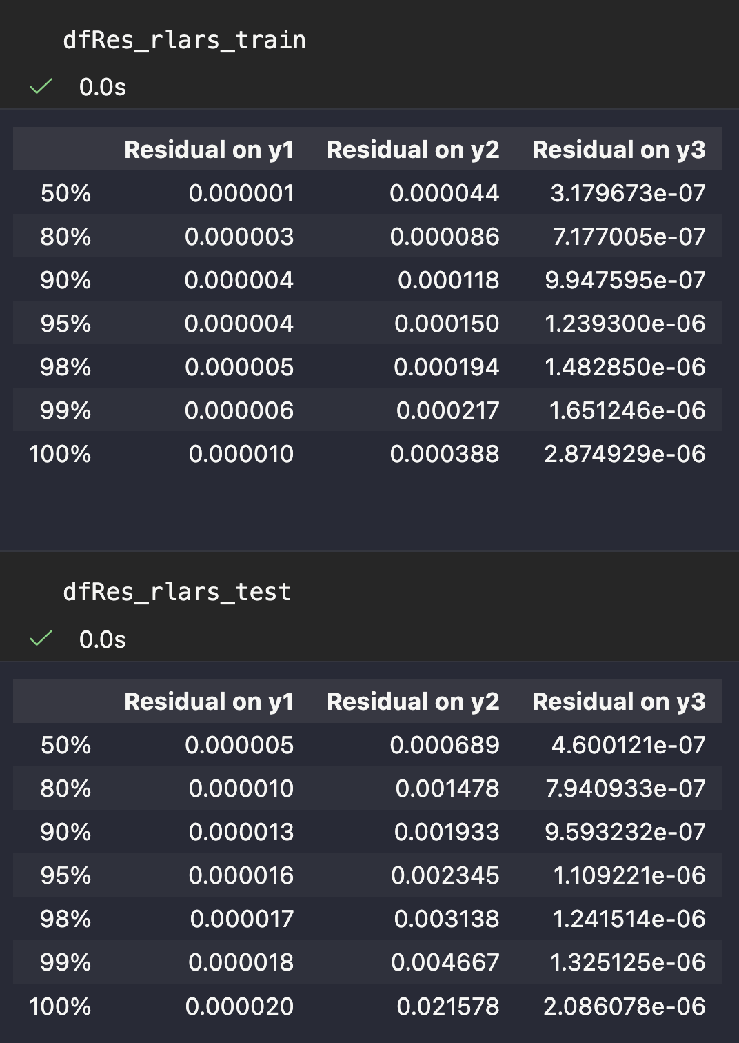
In order to be able to appreciate the generalization power of the model that has been identified using quite small amount of data. It is important de recall the two following facts:
The train/test split has been performed without shuffle with \(\texttt{test\_size}=0.4\) meaning that the first 60% of the scenario is used for the train while the remaining 40% is used to test.
The following figures show the four different scenarios used:
It comes from the observation of the length of each of the four scenarios that the training data concerns almost only the first two experiments while the last two experiments are part of the test data.