PwPol

API documentation

Recall that the objective of the pwpol module is the following:

Given a set of sensors \(s_j\), \(j=1,\dots,n_s\) and a target sensor \(s_i\), find a set of \(n_r\) polynomials \(P_\sigma\), \(\sigma=1,\dots,n_r\), such that the following residual: \[ e_i = \min_{\sigma=1}^{n_r}\Bigl\vert s_i-P_\sigma(\{s_j\}_{j\neq i})\Bigr\vert \tag{1}\] is small.

The principle is similar to the previously presented modules plars and g2sys, the main call needs a dictionary of arguments to be procided which is described in the following section.

1 The `pwpol` arguments dictionary

Here again, as the plars module lies in the heart of all the methods proposed in the Mizopol package, the dictionary unavoidably contains the entries of the plars dictionary and the plars fit dictionary. In particular, the following keys are present that have been already presented in the plars documentation:

deg, nModels, nModes, window, eps, eta coming from the plars’s instance dictionary.
decoule, nfeats, compute_contributions, th_monomial, coming from the plars fit dictionary.

Additional arguments are needed that are linked to the search for the piece-wise polynomial representations.

For the sake of completeness, all the parameters are included in the table below, the old as well as the new ones.

Table 1: Possible entries in the pwpol module args dictionary.

Parameter	Type	Used for	Default
`deg`	`int`	The degree of the polynomial to be identified	`1`
`window`	`int`	number of samples per window (window width)	`200`
`nModels`	`int`	Number of sampled window for alignement evaluation	`10`
`nModes`	`int`	Number of selected monomials per window	`10`
`eps`	`float`	precision for the final least squares solution	`5e-2`
`nBatch`	`int`	Number of window used to determine monomials contributions	`25`
`eta`	`float`	The quantile used to compute the error dataframe	`50`
`th_monomial`	`float`	Threshold to keep a candidate monomial	`1e-4`
`decouple`	`boolean`	Whether to avoid updating the coefficients of the previously selected modes when new ones are selected	`False`
`compute_contributions`	`boolean`	Whether to compute the contributions of monomial for later displaying	`False`
`nfeats`	`int`	Maximum number of sensors to to involve in the solution	`None`
`th`	`float`	Initial value of the precision threshold used to admit a candidate polynomial during the search	`0.1`
`Nguess`	`int`	The number of regions centers that are randomly sampled when searching for regions in the features space	`5`
`Niter`	`int`	The number of solutions for the same centers to account for the randomness of the `plars` solutions	`5`
`ncoef_max`	`int`	The maximum cumulative number of coefficients included in all the retained polynomials	`5000`
`expansion_rate`	`float`	Expansion rate used to increase the precision threshold, initially at `th` after unsuccessful rounds	`1.2`
`ratio_untreated`	`float`	Ratio of the dataset that can be left without being fitted by any polynomial	`0.01`
`dx`	`float`	Initial size of the regions around the randomy sampled center in the space of normalized features.	`0.02`

2 The `fit` method

2.1 Input arguments

Table 2: Input arguments for the fit method of the pwpol module.

Parameter	Type	Used for	Default
`df`	`pandas dataframe`	The dataframe used in the fit	user-defined
`colX`	`list[str]`	The list of columns in `df` to be used as features	user-defined
`coly`	`str`	The column in `df` to be used as label	user-defined
`args`	`dict`	The arguments dictionary discussed in Section 1	user-defined
`plot_conv`	`bool`	If set to `True` a plotly figure is provided showing the convergence log of the solution	`False`

2.2 Returned arguments

Table 3: Input arguments for the fit method of the pwpol module.

Parameter	Type	Description
`model`	`dict`	Dictionary containing all the information defining the model (see below for a complete list)
`cpu`	`tuple`	The tuple of local and distant computation times

The following table enumerates all the fields contained in the returned model.

Table 4: Description of the model dictionary returned by the fit method of the pwpol module.

Parameter	Type	Description
`solutions`	`list[dict]`	The list of `plars` solution representing the polynomials retained in the fitted piece-wise polynomial model
`centers`	`list[list[float]]`	The matrix of centers, each row is a center of a region that was fitted by the polynomial having the same index in `solutions`
`rayons`	`list[float]`	The list of radius of the region around the centers where the polynomial has been identified
`populations`	`list[int]`	The list of integers representing the number of samples contained in the region of the same index
`dens`	`list[float]`	The vector of normalizing coefficients applied to the columns of the training dataframe `df` used for the fit
`log`	`dict`	The log dictionary containing some information regarding the fitting process
`colX`	`list[str]`	The argument `colX` used in the fit (see Table 2)
`coly`	`str`	The argument `coly` used in the fit (see Table 2)
`th`	`float`	The argument `th` used in the fit (see Table 2)
`args`	`dict`	The argument `args` used in the fit (see Table 2)
`deg`	`int`	The argument `deg` used in the arguments dictionary (see Table 1)
`fig_conv`	`plotly \| None`	The convergence figure in case the parameter `plot_conv` of the call is set to `True`
`df_sensitivity`	`pandas dataframe \| None`	The sensitivity dataframe in case `compute_contributions` is set to `True`

2.3 Fit example

from mizopol.pwpol_api import fit

df = pd.read_csv('datasets/Zema.csv', index_col=0).iloc[::5]
coly = 'PS3'
colX = [c for c in df.columns if c != coly]

args = dict(
    th=0.05,
    deg=3,
    window=200,
    compute_contributions=True,
    th_monomial=1e-3,
)

model, (cpu1, cpu2) = fit(df=df[::10], colX=colX, coly=coly,
                            args=args, plot_conv=True)
# let us recover the solutions field fo the model
if 'fig_conv' in model:
    model['fig_conv'].show()

print('\n')
print('arguments of the call:')
print(model['args'], '\n')
print('---------')
print('Sensitivity dataframe:')
print(model['df_sensitivity'], '\n')
print(f'cpu total = {cpu1:1.3} | cpu distance {cpu2:1.3} \n')

print('The list of keys:')
print(model.keys())

Results:

Treated   0% | #rows=   5109 | #models =   0 | #coeffs =   0, | th=0.050
Treated  85% | #rows=    807 | #models =   1 | #coeffs =   4, | th=0.050
Treated  92% | #rows=    427 | #models =   2 | #coeffs =   7, | th=0.050
Treated  95% | #rows=    256 | #models =   3 | #coeffs =  14, | th=0.050
Treated  97% | #rows=    201 | #models =   4 | #coeffs =  33, | th=0.050
Treated  97% | #rows=    201 | #models =   4 | #coeffs =  33, | th=0.050
Treated  97% | #rows=    201 | #models =   4 | #coeffs =  33, | th=0.050
Treated  97% | #rows=    201 | #models =   4 | #coeffs =  33, | th=0.050
Treated  97% | #rows=    201 | #models =   4 | #coeffs =  33, | th=0.050
Treated  98% | #rows=    127 | #models =   5 | #coeffs =  43, | th=0.104


arguments of the call:
{'deg': 3, 'window': 200, 'nModes': 10, 'nModels': 10, 'eps': 0.05, 'nBatch': 25, 'eta': 95, 'dx': 0.02, 'th': 0.05, 'Niter': 5, 'Nguess': 5, 'ncoeff_max': 5000, 'ratio_untreated': 0.01, 'from_dataframe': True, 'th_monomial': 0.001, 'compute_contributions': True, 'decouple': False, 'nfeats': None, 'expansion_rate': 1.2, 'th_percentile': 99.0, 'colX': ['PS1', 'PS2', 'PS4', 'PS5', 'PS6', 'EPS1'], 'coly': 'PS3'} 

---------
Sensitivity dataframe:
      Contribution
PS2       0.347512
PS1       0.293670
EPS1      0.173660
PS5       0.094850
PS4       0.059131
PS6       0.027503
1         0.003675 

cpu total = 32.8 | cpu distance 32.3 

The list of keys:
dict_keys(['solutions', 'centers', 'rayons', 'populations', 'dens', 'log', 'colX', 'coly', 'th', 'args', 'deg', 'inds', 'cpu', 'fig_conv', 'df_sensitivity'])

Notice also since we asked for the convergence plot, the execution of the previous script shows the following plotly figure

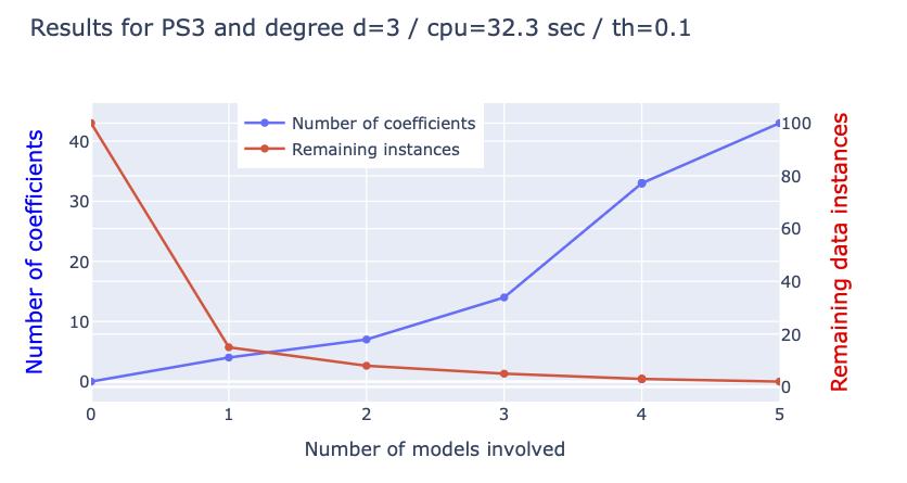
The convergence plot produced by the `pwpol` fitting call. Notice that the print `th` is the last one obtained during the fit and resulting from the expansion when necessary. The value of the initial `th` can be read inside the `model['args']` field.

3 The `predict` method

Once a model is obtained through the fit method, it can be used on a new dataframe to produce prediction. However:

Prediction of a pwpol model

As the model is implicit, the residual defined by Equation 1 can be computed only if the true label y is available. In the absence of the label, only the values of all the polynomials involved in the model can be computed and this does not deliver any residual as each of these value is legitimate candidate as value of the label.

3.1 The `options` dictionary

The availability of the label y is provided to the predict method through the options dictionary (that will be used as one of the input arguments of the predict method) that might be empty or showing one or both of the following fields:

options = None
options = {'y': y, 'n':5}
options = {'n': 5}
options = {'y': y}

in which \(y\) is the true label contained in the dataframe. the n fields might be used to define the number of polynomials to be used. Indeed, as it has been shown in the results of the fit process above, it might happen (and it generally happens) that the last polynomials are used in order to handle a small amount of remaining samples making them not necessarily mandatory for a good fit. that is why the n field in the option dictionary has been introduced.

If the value is None (default value), no residual is computed and the prediction of all the polynomials involved in the model are computed in a matrix Ypred having as many columns as there are polynomials in the model.

3.2 The input arguments

Now that we introduced the option dictionary we can move on to present the input argument of the predict method.

Table 5: Input arguments for the predict method of the pwpol module.

Parameter	Type	Description	Default
`df`	`pandas dataframe`	The dataframe to be used in the prediction	user-defined
`model`	`dict`	The `pwpol` model that is returned by the `fit` method	user-defined
`options`	`dict`	The options dictionary	None

3.3 The returned arguments

Table 6: The returned items by the predict method of the pwpol module.

Parameter	Type	Description
`Ypred`	`list[list[float]]`	The matrix of prediction by all the polynomials in the `model`
`ypred`	`list[float] \| None`	The predicted label in case the `options['y']` is provided, else, None is returned
`dfe`	`pandas dataframe \| None`	The normalized percentile of error in case the `options['y']` is provided, else, None is returned
`ind_polynomial`	`list[int] \| None`	The vector of index of the closest polynomial in case the `options['y']` is provided, else, None is returned
`cpu`	`tuple`	The tuple providing the local and the distant computation times.

3.4 `predict` example

df = pd.read_csv('datasets/Zema.csv', index_col=0).iloc[::5]
coly = 'PS3'
colX = [c for c in df.columns if c != coly]

args = dict(th=0.1,deg=2,window=2000,compute_contributions=True,th_monomial=1e-3)

model, (_,_) = fit(df=df, colX=colX, coly=coly, args=args, plot_conv=False)

options = dict(y = df[coly].values)

#-----------------------------------------------------------------------------
Ypred, ypred, dfe, ind_polynomial, (cpu1, cpu2) = predict(df, model, options)
#-----------------------------------------------------------------------------

plot = True
if plot:
    fig = go.Figure()
    t = np.linspace(0,1, len(ypred))
    fig.add_trace(go.Scatter(x=t, y=ypred, name='predicted'))
    fig.add_trace(go.Scatter(x=t, y=options['y'], name='true'))
    fig.show()

print('percentiles of errors \n', dfe)
print(f"cpu all {cpu1:1.3} | cpu distant {cpu2:1.3}")
print('log')
print('------')
for key, value in model['log'].items():
    print(key, value)
print('------')
print('cardinalities: ', [sol['card'] for sol in model['solutions']])
print('------')
print('Thresholds \n', 'initial = ', model['args']['th'], '| final = ', model['th'])
print('colX = ', model['colX'])

Results:

Treated   0% | #rows=  51084 | #models =   0 | #coeffs =   0, | th=0.100
Treated  96% | #rows=   2077 | #models =   1 | #coeffs =  10, | th=0.100
Treated  96% | #rows=   2077 | #models =   1 | #coeffs =  10, | th=0.100
Treated  97% | #rows=   1535 | #models =   2 | #coeffs =  17, | th=0.120
percentiles of errors 

          Error
50%   0.018472
80%   0.043386
90%   0.059735
95%   0.076548
98%   0.124325
99%   0.207965
100%  1.419767

cpu all 2.44 | cpu distant 0.14

log
------
remain [100, 4, 4, 3]
nb_models [0, 1, 1, 2]
nb_coeff [0, 10, 10, 17]
cpu 87.91623163223267
------
cardinalities: [10, 7]
------
Thresholds 
 initial =  0.1 | final =  0.12
colX =  ['PS1', 'PS2', 'PS4', 'PS5', 'PS6', 'EPS1']

1 The pwpol arguments dictionary

2 The fit method