rlars
labels as roots of a polynomials with features-dependent coefficients.
1 Why?
Despite the fact that single multi-variate polynomials1 is a decently wide class, it obviously does not covre all possible relationships. In particular, rational relationships such as: \[ y = \dfrac{c_0(x)}{c_1(x)} \tag{1}\]
is widely present in the expressions of physical laws.
Think about Euler-Lagrange equations that characterize the majority of mechanical systems where the ineria matrix might depend on the angular positions making the expression of the external torque more in the form of Equation 1 than single polynomials.
the rlars module of the MizoPol suite has been initiated to address this specific case and as a matter of fact, when a pure rational relationship is present, rlars provides an explicit and elegant way to capture it.
Meanwhile, it rapidly came out that in the general case, the identification of the relationships, as it is done in rlars generally leads to \(y\) being a root of a multivariate polynomials of degree \(r\ge 1\) where the coefficients themselves, are polynomials in \(x\).
As a matter of fact, Equation 1 is simple the explicit expression of \(y\) being the root of the polynomial: \[c_1(x)y-c_0(x)\]
and it is only in this case (where the degree \(r=1\)) that \(y\) can be explicitly expressed as a function of the features vector \(x\). In the other cases, any one of the real multiple roots of the polynomial is an eligible candidate to be the value of \(y\).
In this last case (\(r>0\)) the rlars residual provides an implicit characterization of normality. However, this implicit characterization differs from the one provided by the pwpol module (see the dedicated section) in the way the residual is computed. The better choice is obviously problem-dependent.
There is obviously a major difference which is that the number of piece-wise models in rlars cannot exceed the degree of the polynomials as implemented in plars (namely something around \(10\)) while the pwpol module might involved unlimited number of sub-models to capture complex relationships.
In the following section, some more detailed and formal description of the mathematical structure describing the link between the label \(y\) and the vector of features \(x\) as expressed in a model provided by the rlars module is proposed.
2 Mathematical structure
2.1 \(y\) as a root of a polynomial with \(x\)-dependent polynomial coefficients
Given,
- a vector of features \(x\) and
- a label \(y\),
rlars looks for a set of multi-variate polynomials:
\[ c_0(x),\dots, c_r(x) \]
such that \(y\) is a root of the following scalar polyomial (in the unknown \(z\)):
\[ c_r(x)z^r+\dots+c_1(x)z+c_0(x) \]
More precisely, the following can be viewed as a residual for the normality characterization of the pair \((x,y)\):
\[ R(x,y):=c_r(x)y^r+\dots+c_0(x) \tag{2}\]
that can be for instance used in anomaly detection.
Moreover, as it is discussed in the previous section, when \(r=1\), the solution provides an explicit prediction formulae for the label \(y\) as a rational explicit function of the vector of features \(x\).
2.2 Structure of the relationships
In order to get a feeling regarding the class of relationships involved in the general case, some known facts are worth recalling.
Let the polynomial be \[ p(z) = c_{r}(x) z^{r} + c_{r-1} z^{r-1} + \cdots + c_1(x)z + c_0, \] and let its roots be \(z_1, z_2, \ldots, z_{r}\) (which are generally complex numbers).
Then Vieta’s formulas state that: \[ \begin{aligned} z_1 + z_2 + \cdots + z_{r} &= -\frac{c_{r-1}(x)}{c_{r}(x)}, \\ \sum_{1 \le i < j \le r} z_i z_j &= \frac{c_{r-2}(x)}{c_{r}(x)}, \\ \sum_{1 \le i < j < k \le r} z_i z_j z_k &= -\frac{c_{r-3}(x)}{c_{r}(x)}, \\ &\quad \vdots \\ z_1 z_2 \cdots z_{r} &= (-1)^{r} \frac{c_0(x)}{c_{r}(x)}. \end{aligned} \]
This equations underlines the fact that the relationships are mainly composed transformations of rational relationships. This makes them quite rich compared to simple polynomial be it multivariate, and hence suggests that sparser relationships might be so expressed.
At least, this discussion suggests that the two possibly implicit characterization provided by the pwpol and the rlars modules are complementary.
3 Computation flow
In order to clarify the concept of \(y\) being a root of a polynomial with \(x\)-dependent polynomial coefficients and how this can be used to generate residuals, the following Figure gives a graphical representation of the computation flow:
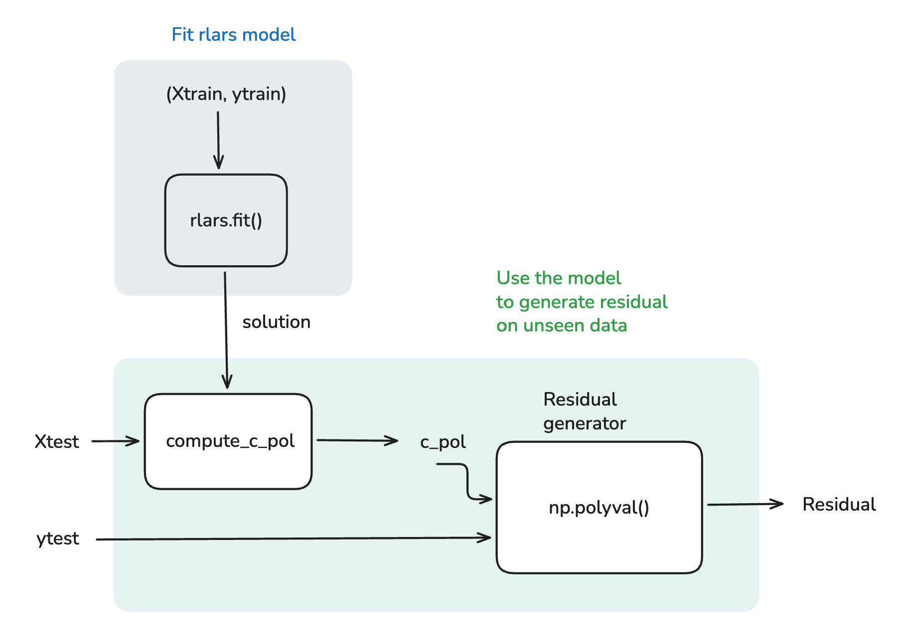
In the following section, an example is provided that illustrates the use of the rlars in designing invariant relationships that hold for the twing pendulum system.
Footnotes
Meaning single multi-variate polynomials and not explicit piece-wise polynomials class which can be viewed as universal and complete class of relationships.↩︎