plars

A tool for sparse identification of polynomial relationships

Before we dig into the details of the plars syntax, calling parameters and the returned outputs as well as a series of use-cases, let us first precisely state the problem it is designed for, as well as the raison d’être of this new algorithm in the first place.

1 Problem statement

The plars module is designed to solve the following regression problem:

Problem statement

Given

a matrix of features $X$ and
a label vector $y$,

the plars module enables to fit a sparse polynomial $P$ s.t. $y\approx P(x)$, namely:

\[ y\approx P(x)=\sum_{i=1}^{n_c} c_i\phi_i(x)\quad\text{where}\quad \phi_i(x) = \prod_{j=1}^{n}x_j^{p_{ij}} \tag{1}\]

By sparse it is meant that the polynomial $P$ is computed in a way that enhances the fact that it involves a small number $n_c$ of monomials with non vanishing coefficients¹ $c_i$.

Leaving sparsity apart, this is obviously a linear problem in the parameter vector $c=(c_1,\dots, c_{n_c})$ and hence can be viewed as a rather tractable problem.

As a matter of fact, the genesis of the mizopol suite lies in the fact that:

The curse of dimensionality

In the industrial context, it is not uncommon to have datasets that involves a large number of sensors, say 50 or even much larger numbers.

In such cases, considering high multi-variate polynomials with high degrees might induce a number of candidate monomials that increases quite rapidely.

This might lead to a number of unknowns that can reach hunderds of thousands.

This is explained in the next section.

2 Cardinality of multivariate polynomials

The number of eligible monomials $\phi_i$ in definition (see Equation 1) of a polynomial $P$ in $n$ variables and degree $d$ is given by the formulae²:

\[ n_c = \begin{pmatrix} n+\text{deg}\\ \text{deg} \end{pmatrix} \]

The following figure shows typical values of $n_c$ for different values of the pair $(n,d)$:

Figure 1: Number of candidate monomials for different values of the pair $(n,d=\text{deg})$

From the above table it comes out that in the industrial context, the underlying linear problem becomes high dimensional leading to a high risk of overfitting when moderate sizes of training datasets are used which is not uncommon in the industrial world.

This is where sparsity becomes crucial in deriving robust solutions and retrieving the true hidden relationship between physical entities.

Now this being said, the problem stated above (see Section 1) can still be addressed using the well known sklearn.linear.lassolarsCV modules (Pedregosa et al., 2011) or similar ones of the same library³, right?

This is what I thought, initially and it is only when this was not successful for a number of candidate monomials that goes beyond 35000 that the idea of attempting a scalable version came to me and the plars module emerged, together with all the tools based on it which are included in the mizopol suite.

A benchmark has been created (Alamir, 2025) for a fair compaison whose results are sketched in the following section.

3 Comparison with alternative approaches

Let us first define the benchmark used in the comparison (Alamir, 2025).

3.1 The benchmark

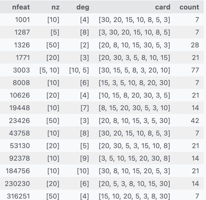
A set of values of $n$ (number of features) is defined

\[ n\in \{5, 10, 20, 50\} \]

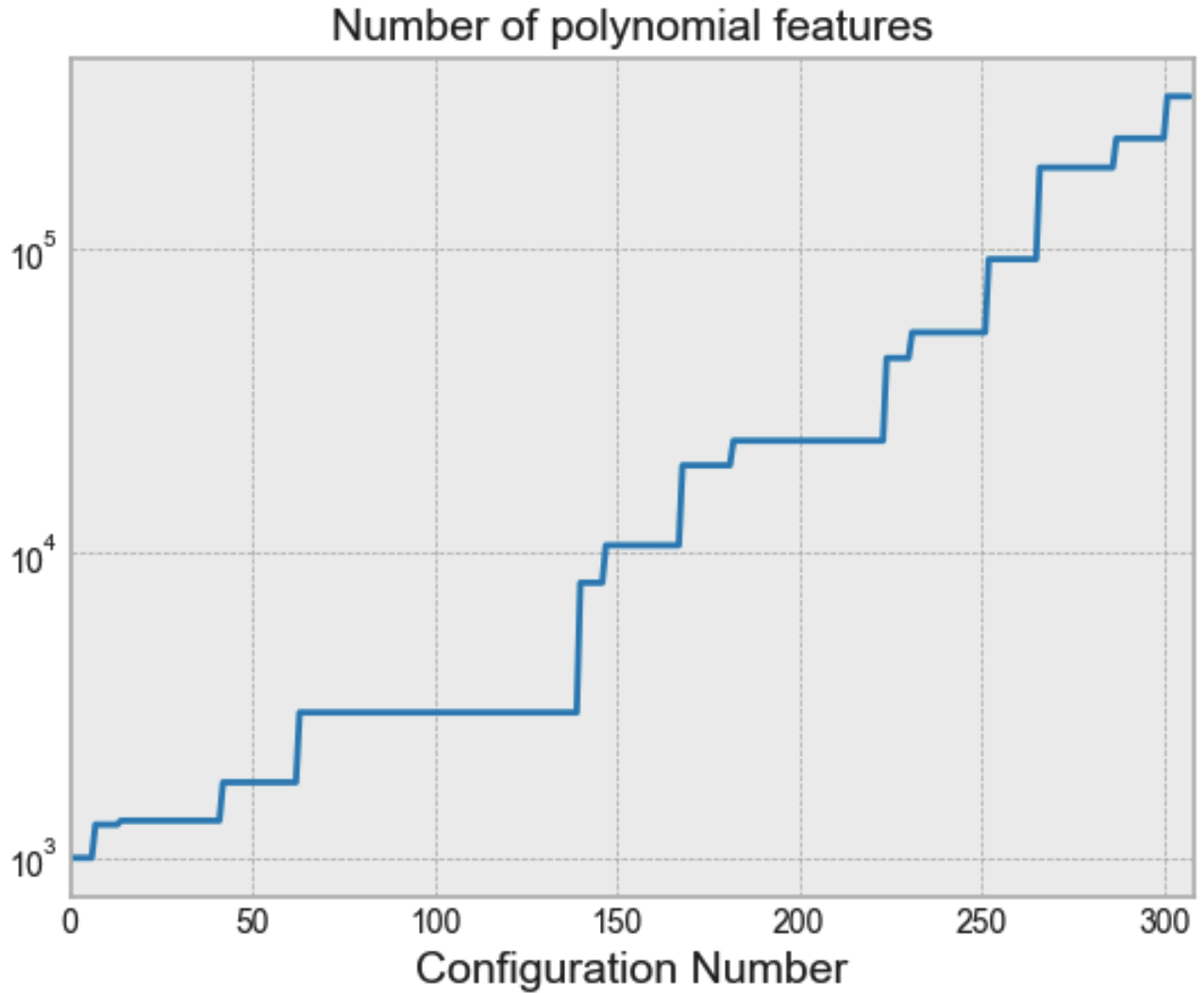
A set of targeted numbers of polynomial features $n_\text{feat}$ is defined

\[ n_\text{feat}\in \{2, 5, 10, 20, \dots, 400\}\times 1000 \]

A set of effective numbers of monomials (those with non zero $c_i$) is defined:

\[ \texttt{card}\in \{3, 5, 8, 10, 15, 20, 30\} \]

A features matrix $X$ is generated

\[ X\in \mathbb R^{100000\times 200} \]

For each scenario $(n,n_\text{feat})$, choose several (random) settings:

\[ \begin{align} &\Bigl\{d^{(j)}\in \mathbb \{0,\dots,d_{max}\}^{n_z}\Bigr\}_{j=1}^{\texttt{card}}\\ &c_i\in \{-1,+1\}^{\texttt{card}} \end{align} \]

Compute \[y = \sum_{i=1}^{\texttt{card}}\Bigl[c_i\underbrace{\prod_{j=1}^{n_x}X[:,j]^{d_{i}^{(j)}}}_\text{\color{MidnightBlue} Monomial $\phi_i(x^{(j)})$}\Bigr] \]

Detailed characteristics of the scenarios.

Percentile of the number of polymial features accross the scenarios.

**Regression error**: (For instance, $e_y=0.1$ means that 95% of the errors are 10 times lower than the median).

**Coefficients reconstruction error**: (Recall that the components of $c$ lie in $[-1,1]$.)

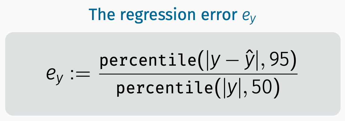
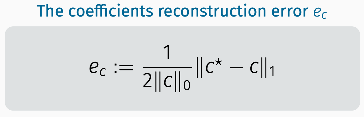
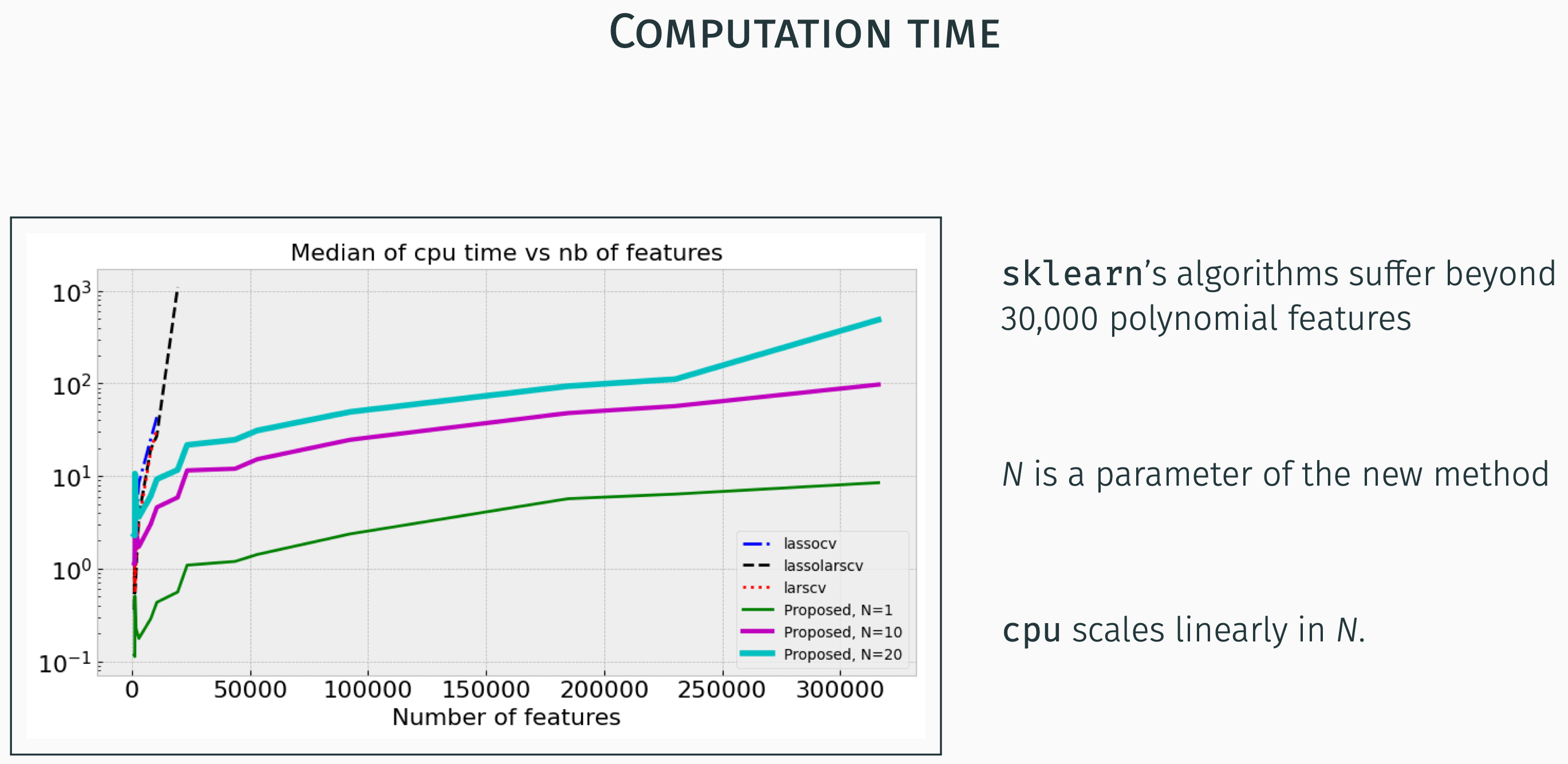
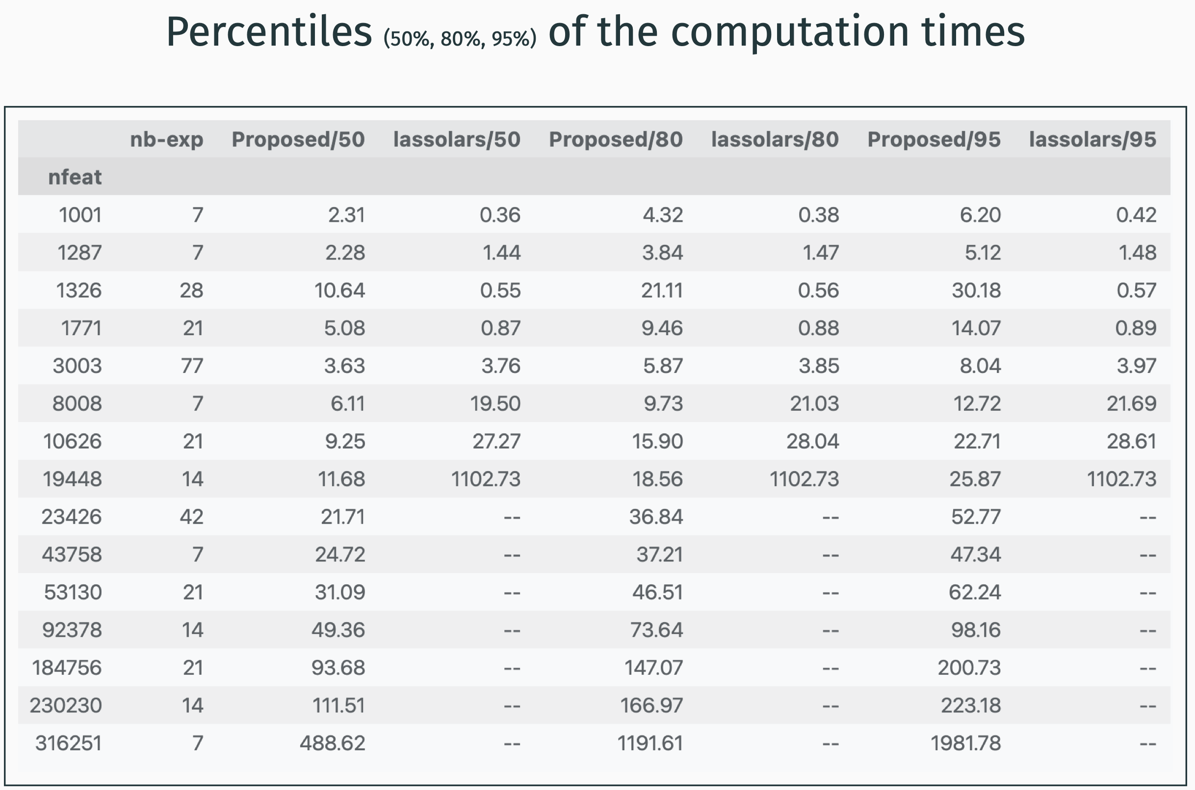
In the graphics below, the plars is referred to with the Proposed, N=? label. N here refers to the number of trials before delivering the results.

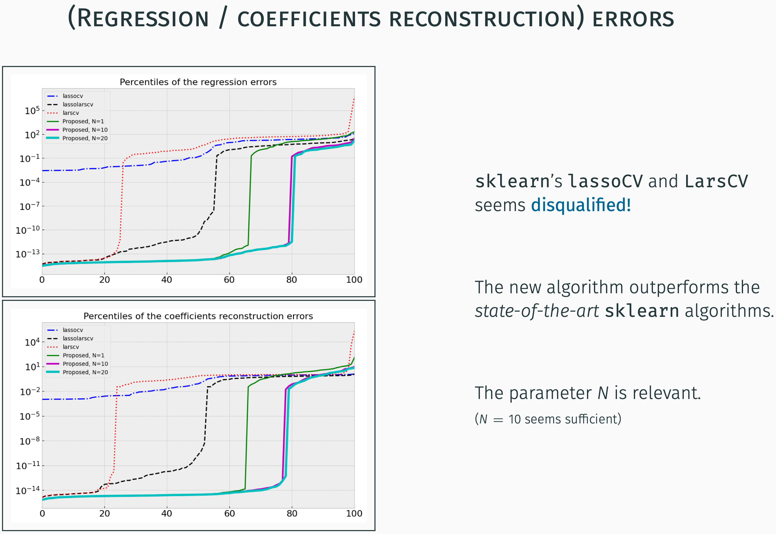
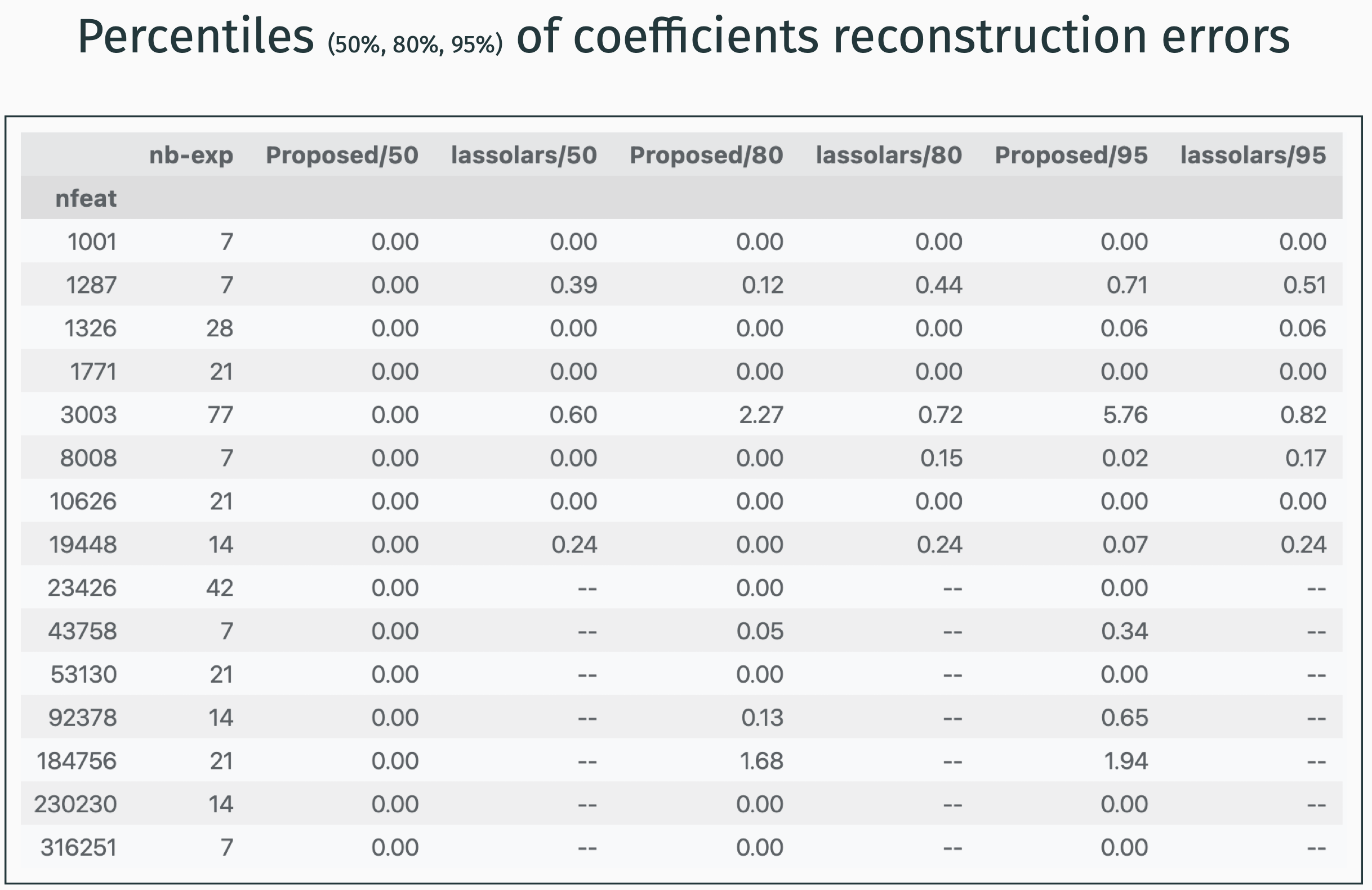
In the next section, the principle of the plars algorithm is sketched.

References

Alamir, M. (2025). Nonlinear control of uncertain systems: Conventional and data-driven alternative with python. Springer-Nature.

Pedregosa, F., Varoquaux, G., Gramfort, A., Michel, V., Thirion, B., Grisel, O., Blondel, M., Prettenhofer, P., Weiss, R., Dubourg, V., Vanderplas, J., Passos, A., Cournapeau, D., Brucher, M., Perrot, M., & Duchesnay, E. (2011). Scikit-learn: Machine learning in Python. Journal of Machine Learning Research, 12, 2825–2830.

Footnotes

See the definition of a polynomial.↩︎
This can be computed by the python math.comb function of the math module.↩︎
After applying a PolynomialFeatures transformation.↩︎